Availability#
This blog is part of a series on robust system design. Check the other posts that address scalability, failures, latency and integration.
Introduction#
In today’s digital landscape, where businesses and users expect seamless, uninterrupted access to services, ensuring high system availability is a critical concern for IT organizations. Modern IT systems comprise numerous interdependent components that exchange information, and their collective availability directly impacts the overall user experience and business continuity.
Key Availability Metrics#
To quantify and measure system availability, several key metrics are commonly used, the graph below is an example of a typical availability graph.
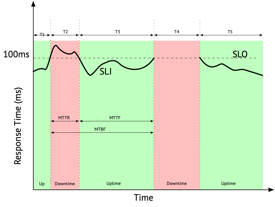
- Service Level Indicator (SLI)
- A quantitative measure that reflects the level of service provided by a system or application. SLIs are typically based on metrics that measure the performance of a service from the user’s perspective. These metrics are usually collected by probes external to the system that imitate user behavior.
- In the graph above, the defined SLI is the average response time of successful requests. Failed or timed out requests are not included in the average. However, the lack of measurements is considered as a total failure and a downtime.
- Synthetic SLI
- An SLI calculated from multiple simple SLIs as defined above.
- A single SLI is usually not enough to properly evaluate a whole application. We probably want to make sure that multiple APIs are responding within an acceptable period AND the failure rate of each of those APIs is more than a certain value.
- Service Level Objective (SLO)
- The acceptable SLI value beyond which the service is considered to be degraded.
- In the graph above, the defined SLO is set at 100 ms.
- Mean Time To Failure (MTTF)
- How long the systems behaves as expected before failure. In SaaS systems, this is also called Uptime. This is the mean time interval where $$ SLI>SLO $$
- In our example periods T1, T3 and T5 are considered as uptime so the MTTF is
$$ MTTF=\frac{T1+T3+T5}{3}=\frac{3+12+11}{3}=8.67h $$
- Mean Time To Repair (MTTR)
- How long it takes to repair the system after failure, this includes troubleshooting the problem, replacing a part, restarting a component or failing over to a redundant system. This figure can be very hard to estimate. In SaaS systems, this is also called Downtime and is measured as the mean time interval where $$ SLI<SLO $$
- In our example, T2 and T4 are downtime periods so the MTTR is
$$ MTTR=\frac{T2+T4}{2}=\frac{5+9}{2}=7h$$
- Availability
- Percentage of time the system is available to the user.
- $$ Availability = \frac{MTBF}{MTBF + MTTR} = \frac{uptime}{uptime + downtime} $$
- In our case, the total availability of the system is
$$ Availability = \frac{T1+T3+T5}{T1+T2+T3+T4+T5} = \frac{3+13+11}{40} = \frac{26}{40} = 0.65 = 65% $$
- Failure
- Percentage of time the system is not performing as expected
- $$ Failure = \frac{MTTR}{MTBF + MTTR} = \frac{downtime}{uptime + downtime} = 1 - Availability $$
- In our case, the total failure of the system is
$$ Failure = \frac{T2+T4}{T1+T2+T3+T4+T5} = \frac{5+9}{40} = \frac{14}{40} = 0.35 = 35%$$
Measuring availability#
Use external probes to measure SLIs and push the metrics to a central instance which will graph the individual SLIs and calculate a synthetic SLI and the total system availability.
The open-source kuvasz-agent can probe multiple endpoints with specific headers and measure response time and success rates. It can push these metrics to a self-hosted Grafana/Mimir instance and thus have a fully free and open-source solution.
It is a good idea to have probes in geographical locations of real users and using the access networks these users will actually use. If an application target is to be used during peak hours from a mobile network, the best probe is a Mobile Data modem connected to a machine and simulating client calls.
Availability classes#
Total system availability is usually expressed as a number of nines as in the following table.
| Nines | Availability | Downtime per year |
|---|---|---|
| 1 | 90% | 36.53 days |
| 2 | 99% | 3.65 days |
| 3 | 99.9% | 8.77 hours |
| 4 | 99.99% | 52.60 minutes |
| 5 | 99.999% | 5.26 minutes |
| 6 | 99.9999% | 31.56 seconds |
Architecture and availability#
In order to think about the availability of a system, it is usually useful to break it down into components and think about the availability of each component.
There are usually two ways to compose systems:
Serial composition#
Break the functionality in two components where component 1 performs part of the functionality and hands over to component 2 to perform the other part. In this case, the availability of the system is the availability of component 1 multiplied by the availability of component 2.
$$ Availability = Availability_1 * Availability_2 $$
As an example, consider a typical web system consisting of a web server, an application server and a database.
flowchart LR
  S((Browser)) --> A[Web Server]
  subgraph System
  A --> B[Application Server]
  B --> C[Database Server]
  end
If each system has an availability of $$ A $$ then the availability of the system is $$ A^3 $$.
To put things in perspective, if each of the above servers has an availability of four nines or 99.99% then then the availability of the system is $$ 99.99%^3 = 0.9999^3 = 0.9997 = 99.97% $$
So the average downtime of the system has gone up from
$$ 52.6\ minutes = 0.88\ hours $$
to
$$ (1-.9997) * 365.25 * 24 * 60 = 157.68\ minutes = 2.63\ hours$$
or a threefold increase.
Parallel composition#
Duplicate the system and let the users balance the load among the two components. In this case, the availability of the system is calculated using the following formula as you need both systems down for the service to be down.
$$ Availability = 1 - (1 - Availability_1) * (1 - Availability_2) $$
As an example, consider a scaled web server
flowchart LR
  S((Browser)) --> A[Load Balancer]
  subgraph System
  B1
  B2
  B3
  end
  A --> B1[Web Server 1]
  A --> B2[Web Server 2]
  A --> B3[Web Server 3]

  B1 --> C[Application Server]
  B2 --> C
  B3 --> C
  C --> E[Database Server]
In this case, if the availability of each server is 99.99% then the availability of the system consisting of the three web servers is
$$ 1 - (1 - 0.9999)^3 = 1 - 0.0001^3 = 0.999999999999 = 99.9999999999% $$
In other words, availability has gone up from four nines to twelve nines.
Conclusion#
While high availability is desirable, achieving it often comes with increased costs, including hardware redundancy, software licenses, and operational complexity.
The rules to maximize availability while optimizing resources are:
A1. Minimize the number of serial components
A2. Have at least two or three parallel components